格物
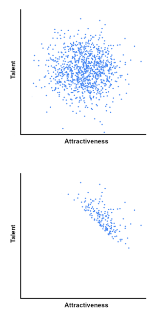
图:Belbury · CC0 · Wikimedia Commons
伯克森悖论
Berkson's paradox
tendency to misinterpret statistical experiments involving conditional probabilities
伯克森悖论,又称伯克森偏差、碰撞偏差或伯克森谬误,是指人们的直觉观察与实际上真实的条件概率和严谨的统计结果不相符,也就是说人们所发现的看似两个相关的因素实际上根本无关。当研究设计中纳入偏差样本以及存在偏差的情况下就会出现这种情况。这一悖论由美国医生和统计学家约瑟夫·伯克森于1946年提出。
摘自维基百科「伯克森悖论」,CC BY-SA 4.0
- 类型
- 悖论、认知偏误
- 命名来源
- 约瑟夫·伯克森
- 上级概念
- 悖论、认知偏误
百科正文
英文维基百科补充中文条目比较短,下面是英文条目「Berkson's paradox」的原文
Berkson's paradox, also known as Berkson's bias, collider bias, endogenous selection bias or Berkson's fallacy, is a result in conditional probability and statistics which is often found to be counterintuitive, and hence a veridical paradox. It is a complicating factor arising in statistical tests of proportions. Specifically, it arises when there is a sampling bias inherent in a study design. The effect is related to the explaining away phenomenon in Bayesian networks, and conditioning on a collider in graphical models.
This paradox is often illustrated using scenarios from the fields of medical statistics or biostatistics, as in the original description of the problem by Joseph Berkson.
The most common example of Berkson's paradox is a false observation of a negative correlation between two desirable traits, i.e., that members of a population which have some desirable traits tend to lack a second. Berkson's paradox occurs when this observation appears true when in reality the two properties are unrelated—or even positively correlated—because members of the population where both are absent or not equally observed. For example, a person may observe from their experience that attractive celebrities tend to be untalented, and talented celebrities unattractive; but people who are neither particularly talented nor attractive will not become celebrities, so will not be part of the observer's perspective.
Examples
Original illustration
Berkson's original illustration involves a retrospective study examining a risk factor for a disease in a statistical sample from a hospital in-patient population. Because samples are taken from a hospital in-patient population, rather than from the general public, this can result in a spurious negative association between the disease and the risk factor.
For example, if the risk factor is diabetes and the disease is cholecystitis, a hospital patient without diabetes is more likely to have cholecystitis than a member of the general population, since the patient must have had some non-diabetes (possibly cholecystitis-causing) reason to enter the hospital in the first place. That result will be obtained regardless of whether there is any association between diabetes and cholecystitis in the general population.
Dating pool example
An example presented by mathematician Jordan Ellenberg is that of a dating pool, measured on axes of niceness and handsomeness. A person might conclude from their own dating experience that "the handsome ones tend not to be nice, and the nice ones tend not to be handsome".
Suppose Alice will only date men whose niceness plus handsomeness exceeds some threshold. Then nicer men do not have to be as handsome to qualify for her dating pool. So, among the men that Alice dates, the nicer ones are less handsome on average (and vice versa), even if these traits are uncorrelated in the general population.
This does not mean that men in the dating pool compare unfavorably with men in the population.
Statement
Two independent events become conditionally dependent given that at least one of them occurs. Symbolically:
- If P(A∩ B)=P(A)P(B) and P(A∪ B)<1 then P(A∩ B| A∪ B)<P(A| A∪ B)P(B| A∪ B)
- Proof: Note that P(A| A∪ B)=P(A)/P(A∪ B) and P(B| A∪ B)=P(B)/P(A∪ B)
- which, together with P(A∩ B)=P(A)P(B) and P(A∪ B)<1 (so (公式略)) implies that (公式略)
One can see this in tabular form as follows: the yellow regions are the outcomes where at least one event occurs (and ~A means "not A").
For instance, if one has a sample of 100, and both A and B occur independently half the time ( P(A)=P(B)=1/2), one obtains:
So in 75 outcomes, either A B occurs, of which 50 have A occurring. By comparing the conditional probability of A to the unconditional probability of A: P(A| A∪ B)=50/75=2/3>P(A)=50/100=1/2
We see that the probability of A is higher ( 2/3) in the subset of outcomes where ( A or B) occurs, than in the overall population ( 1/2). On the other hand, the probability of A given both B and ( A or B) is simply the unconditional probability of A, P(A), since A is independent of B. In the numerical example, we have conditioned on being in the top row:
Here the probability of A 25/50=1/2.
以上节选摘自英文维基百科「Berkson's paradox」,按 CC BY-SA 4.0 使用,去掉了参考文献、外部链接等尾部小节,公式改写成了纯文本。篇幅所限,较长的小节只摘了开头一部分,有的小节没有收;全文、配图和出处见原文。