常数变易法1766

对于一阶非齐次线性微分方程，通常可以通过积分因子或待定系数以相当少的努力找到解，尽管这些方法利用涉及猜测的启发式方法并且不适用于所有非齐次线性微分方程。

参数的变化也扩展到线性偏微分方程，特别是线性演化方程的非齐次问题，如热方程、波动方程和振动板方程。 在这种情况下，该方法通常被称为杜哈梅原理，以首先应用该方法求解非均匀热方程的法国数学家让-玛丽·杜哈梅（1797-1872）的名字命名。 有时参数本身的变化称为杜哈梅原理，反之亦然。

In mathematics, variation of parameters, also known as variation of constants, is a general method to solve inhomogeneous linear ordinary differential equations.

For first-order inhomogeneous linear differential equations it is usually possible to find solutions via integrating factors or undetermined coefficients with considerably less effort, although those methods leverage heuristics that involve guessing and do not work for all inhomogeneous linear differential equations.

Variation of parameters extends to linear partial differential equations as well, specifically to inhomogeneous problems for linear evolution equations like the heat equation, wave equation, and vibrating plate equation. In this setting, the method is more often known as Duhamel's principle, named after Jean-Marie Duhamel (1797–1872) who first applied the method to solve the inhomogeneous heat equation. Sometimes variation of parameters itself is called Duhamel's principle and vice versa.

History

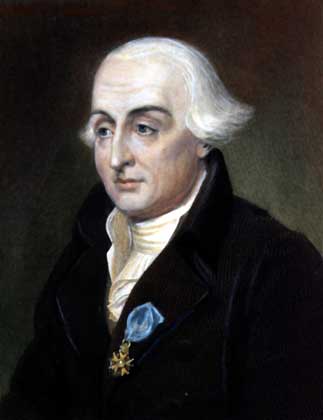
The method of variation of parameters was first sketched by the Swiss mathematician Leonhard Euler (1707–1783), and later completed by the Italian-French mathematician Joseph-Louis Lagrange (1736–1813).

A forerunner of the method of variation of a celestial body's orbital elements appeared in Euler's work in 1748, while he was studying the mutual perturbations of Jupiter and Saturn. In his 1749 study of the motions of the earth, Euler obtained differential equations for the orbital elements. In 1753, he applied the method to his study of the motions of the moon.

Lagrange first used the method in 1766. Between 1778 and 1783, he further developed the method in two series of memoirs: one on variations in the motions of the planets and another on determining the orbit of a comet from three observations.

Description of method

Given an ordinary non-homogeneous linear differential equation of order n

Let y₁(x),…,yₙ(x) be a basis of the vector space of solutions of the corresponding homogeneous equation

• Then a particular solution to the non-homogeneous equation is given by
• where the cᵢ(x) are differentiable functions which are assumed to satisfy the conditions
• Starting with (iii), repeated differentiation combined with repeated use of (iv) gives
• One last differentiation gives
• By substituting (iii) into (i) and applying (v) and (vi) it follows that

The linear system (iv and vii) of n equations can then be solved using Cramer's rule yielding （公式略）

where W(x) is the Wronskian determinant of the basis y₁(x),…,yₙ(x) and Wᵢ(x) is the Wronskian determinant of the basis with the i-th column replaced by (0,0,…,b(x)).

The particular solution to the non-homogeneous equation can then be written as （公式略）

Intuitive explanation

Consider the equation of the forced dispersionless spring, in suitable units: x''(t)+x(t)=F(t).

Here x is the displacement of the spring from the equilibrium x = 0, and F(t) is an external applied force that depends on time. When the external force is zero, this is the homogeneous equation (whose solutions are linear combinations of sines and cosines, corresponding to the spring oscillating with constant total energy).

We can construct the solution physically, as follows. Between times t=s and t=s+ds, the momentum corresponding to the solution has a net change F(s) ds (see: Impulse (physics)). A solution to the inhomogeneous equation, at the present time t > 0, is obtained by linearly superposing the solutions obtained in this manner, for s going between 0 and t.

Examples

First-order equation： y'+p(x)y=q(x)

The complementary solution to our original (inhomogeneous) equation is the general solution of the corresponding homogeneous equation (written below): y'+p(x)y=0

This homogeneous differential equation can be solved by different methods, for example separation of variables: d/dxy+p(x)y=0

• dy/dx=-p(x)y
• （公式略）
• ∫ ∫ 1/y dy=-∫ p(x) dx
• ln |y|=-∫ p(x) dx+C
• y=± e^(-∫ p(x) dx+C)=C₀e^(-∫ p(x) dx)
• The complementary solution to our original equation is therefore: y_(c)=C₀e^(-∫ p(x) dx)
• Now we return to solving the non-homogeneous equation: y'+p(x)y=q(x)

Using the method variation of parameters, the particular solution is formed by multiplying the complementary solution by an unknown function C(x): yₚ=C(x)e^(-∫ p(x) dx)